Tutorial: A Simple Pipeline

The following illustrates how a pipeline like the one above is built using gunpowder. We will build the pipeline incrementally and see what effect each change has. Therefore, this tutorial is best read in that order. Nevertheless, feel free to jump ahead to any of the following topics we are covering here:

To rerun the example given here yourself, have a look at the following preliminaries (or simply head over to this tutorial’s Colab notebook):

Tutorial Preliminaries: Data Preparation and Helpers

To follow the example here, install those packages:

pip install gunpowder
pip install zarr
pip install matplotlib

import matplotlib.pyplot as plt
import numpy as np
import random
import zarr
import torch
from skimage import data
from skimage import filters

# make sure we all see the same
torch.manual_seed(1961923)
np.random.seed(1961923)
random.seed(1961923)

# open a sample image (channels first)
raw_data = data.astronaut().transpose(2, 0, 1)

# create some dummy "ground-truth" to train on
gt_data = filters.gaussian(raw_data[0], sigma=3.0) > 0.75
gt_data = gt_data[np.newaxis,:].astype(np.float32)

# store image in zarr container
f = zarr.open('sample_data.zarr', 'w')
f['raw'] = raw_data
f['raw'].attrs['resolution'] = (1, 1)
f['ground_truth'] = gt_data
f['ground_truth'].attrs['resolution'] = (1, 1)

# helper function to show image(s), channels first
def imshow(raw, ground_truth=None, prediction=None):
  rows = 1
  if ground_truth is not None:
    rows += 1
  if prediction is not None:
    rows += 1
  cols = raw.shape[0] if len(raw.shape) > 3 else 1
  fig, axes = plt.subplots(rows, cols, figsize=(10, 4), sharex=True, sharey=True, squeeze=False)
  if len(raw.shape) == 3:
    axes[0][0].imshow(raw.transpose(1, 2, 0))
  else:
    for i, im in enumerate(raw):
      axes[0][i].imshow(im.transpose(1, 2, 0))
  row = 1
  if ground_truth is not None:
    if len(ground_truth.shape) == 3:
      axes[row][0].imshow(ground_truth[0])
    else:
      for i, gt in enumerate(ground_truth):
        axes[row][i].imshow(gt[0])
    row += 1
  if prediction is not None:
    if len(prediction.shape) == 3:
      axes[row][0].imshow(prediction[0])
    else:
      for i, gt in enumerate(prediction):
        axes[row][i].imshow(gt[0])
  plt.show()

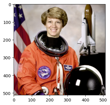
The data we are working with is shown below. It is stored in a zarr container sample_data.zarr in dataset called raw, which has one attribute resolution = (1, 1):

imshow(zarr.open('sample_data.zarr')['raw'][:])

Note

The resolution attribute in the zarr dataset will be read by gunpowder. gunpowder supports anisotropic resultions and even datasets with different resolutions in the same pipeline. Here, it tells gunpowder that this is a 2D dataset, with the remaining dimension to be interpreted as channels. More on this later.

A minimal pipeline

The first step for every pipeline is to declare the arrays that will be used. For now, we will need only one array which we call raw:

import gunpowder as gp

# declare arrays to use in the pipeline
raw = gp.ArrayKey('RAW')

Next we assemble the pipeline itself. To illustrate how gunpowder works, we will do this step by step and look at the changes each step introduces. We start with a “pipeline” consisting only of a data source.

# create "pipeline" consisting only of a data source
source = gp.ZarrSource(
    'sample_data.zarr',  # the zarr container
    {raw: 'raw'},  # which dataset to associate to the array key
    {raw: gp.ArraySpec(interpolatable=True)}  # meta-information
)
pipeline = source

The pipeline by itself does nothing until we request data from it. What exactly is requested is specified by a BatchRequest. The following shows how to create a request for “raw” data, starting at (0, 0) with a size of (64, 64).

# formulate a request for "raw"
request = gp.BatchRequest()
request[raw] = gp.Roi((0, 0), (64, 64))

The request behaves like a dictionary, mapping each array key to a region of interest (ROI), i.e., an offset and a size.

It remains to build the pipeline and request a Batch:

# build the pipeline...
with gp.build(pipeline):

  # ...and request a batch
  batch = pipeline.request_batch(request)

# show the content of the batch
print(f"batch returned: {batch}")
imshow(batch[raw].data)

batch returned: 
	RAW: ROI: [0:64, 0:64] (64, 64), voxel size: (1, 1), interpolatable: True, non-spatial: False, dtype: uint8, placeholder: False

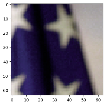
The returned batch contains a crop of the source image, located in the top left corner. This is indeed exactly what we requested, as an inspection of our request reveals:

print(request)

	RAW: ROI: [0:64, 0:64] (64, 64), voxel size: None, interpolatable: None, non-spatial: False, dtype: None, placeholder: False

As we can see, the request for RAW (the name we gave to our array key) is for a ROI that begins at 0 and ends at 64 for each dimension, giving it a shape of (64, 64). The ZarrSource simply delivered on exactly this request.

Further Example: Change Request Offset

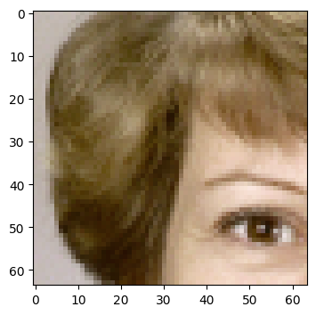
To create a request for data in a specific area of the source, we simply change the offset in the request Roi:

request[raw] = gp.Roi((50, 150), (64, 64))
#                     ^^^^^^^^^
#                     changed offset

with gp.build(pipeline):
  batch = pipeline.request_batch(request)

print(f"batch returned: {batch}")
imshow(batch[raw].data)

batch returned: 
	RAW: ROI: [50:114, 150:214] (64, 64), voxel size: (1, 1), interpolatable: True, non-spatial: False, dtype: uint8, placeholder: False

Random samples

In training pipelines, however, it might be useful to randomly select a location to crop data from. Doing this manually by changing the offset of the ROI in the request we send for every iteration would be cumbersome. It would also require that we know the size of the data in the source.

Instead, gunpowder provides a node RandomLocation that does that for us, we simply have to add it to our pipeline:

# add a RandomLocation node to the pipeline to randomly select a sample

random_location = gp.RandomLocation()
pipeline = source + random_location

print(pipeline)

ZarrSource[sample_data.zarr] -> RandomLocation

When we now issue the same request, it will first be shifted by random_location to a random location within the provided data.

with gp.build(pipeline):
  batch = pipeline.request_batch(request)

imshow(batch[raw].data)

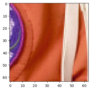
This example illustrates two important concepts in gunpowder:

1. Request can (and will be) changed as they are passed upstream through the pipeline. In this example, RandomLocation changes the offset of the request for us, such that we get data from a random location.

2. gunpowder nodes know what kind of data is provided upstream, and what its extents are. Here, RandomLocation uses this information to find out where it can safely shift the request to.

Geometric augmentation

gunpowder provides many more nodes to be added to a pipeline, most of them tailored towards training pipelines. The following example shows how to add simple random mirror and transpose augmentations:

simple_augment = gp.SimpleAugment()
pipeline = source + random_location + simple_augment

with gp.build(pipeline):
  batch = pipeline.request_batch(request)

imshow(batch[raw].data)

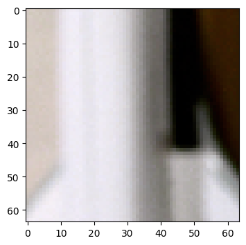
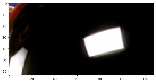
The SimpleAugment node will (by default) randomly mirror and/or transpose batches passing through it. Notably, the transpose operation is transparent, i.e., if we were to request data in a non-square ROI, we will still get the size we asked for, transposed or not:

request[raw] = gp.Roi((0, 0), (64, 128))

with gp.build(pipeline):
  batch = pipeline.request_batch(request)

imshow(batch[raw].data)

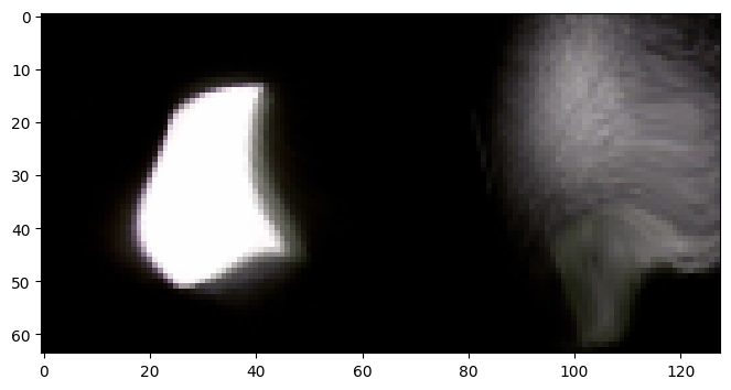
Simple augmentations like this are complemented by random rotations and elastic deformations, which are provided by the ElasticAugment node:

import math

elastic_augment = gp.ElasticAugment(
  control_point_spacing=(16, 16),
  jitter_sigma=(4.0, 4.0),
  rotation_interval=(0, math.pi/2))
pipeline = source + random_location + simple_augment + elastic_augment

with gp.build(pipeline):
  batch = pipeline.request_batch(request)

imshow(batch[raw].data)

Intensity augmentation

Intensity values can be modified and random noise added in a similar fashion:

normalize = gp.Normalize(raw)
intensity_augment = gp.IntensityAugment(
  raw,
  scale_min=0.8,
  scale_max=1.2,
  shift_min=-0.2,
  shift_max=0.2)
noise_augment = gp.NoiseAugment(raw)

pipeline = (
  source +
  normalize +
  random_location +
  simple_augment +
  elastic_augment +
  intensity_augment +
  noise_augment)

with gp.build(pipeline):
  batch = pipeline.request_batch(request)

imshow(batch[raw].data)

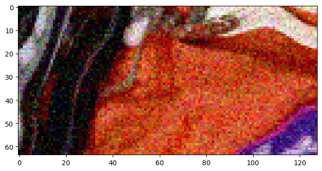
We introduced two new concepts in this snippet:

First, we added a Normalize node for raw. This node ensures that the data type of the given array is np.float from there on through the pipeline. We have so far been agnostic about the exact datatype of raw (it was uint8, by the way). However, in order to shift intensities and to add random noise, it is helpful to ensure we are dealing with float values between 0 and 1. The normalization applied by Normalize is data independent, it is based on the data type of the source (or, optionally, on a user-specified scaling factor).

Second, we introduced nodes that take array keys as arguments (Normalize, IntensityAugment, and NoiseAugment). Those nodes limit their operation to the given keys, which is useful if our batch also contains other arrays (like a ground-truth segmentation) that we do not wish to modify.

Creating batches with multiple samples

So far we have seen how to request a single sample in a “batch”. Normally, however, batches consist of several samples drawn independently. This can be done using the Stack node:

stack = gp.Stack(5)
pipeline = (
  source +
  normalize +
  random_location +
  simple_augment +
  elastic_augment +
  intensity_augment +
  noise_augment +
  stack)

with gp.build(pipeline):
  batch = pipeline.request_batch(request)

imshow(batch[raw].data)

Requesting multiple arrays

To train a model on data, we need a training signal as well. This signal can come, for example, in the form of a binary segmentation stored alongside the raw image data. For this tutorial, we will assume that such a binary segmentation exists and is stored in the same zarr container in a dataset called ground_truth. At the beginning of this tutorial, we created a dummy segmentation to work with:

imshow(
  zarr.open('sample_data.zarr')['raw'][:],
  zarr.open('sample_data.zarr')['ground_truth'][:])

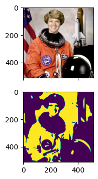
With a slight modification to the source node and our request, we can now simultaneously request raw data and a segmentation:

gt = gp.ArrayKey('GROUND_TRUTH')

source = gp.ZarrSource(
    'sample_data.zarr',
    {
      raw: 'raw',
      gt: 'ground_truth'
    },
    {
      raw: gp.ArraySpec(interpolatable=True),
      gt: gp.ArraySpec(interpolatable=False)
    })

request[gt] = gp.Roi((0, 0), (64, 128))

pipeline = (
  source +
  normalize +
  random_location +
  simple_augment +
  elastic_augment +
  intensity_augment +
  noise_augment +
  stack)

with gp.build(pipeline):
  batch = pipeline.request_batch(request)

imshow(batch[raw].data, batch[gt].data)

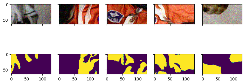
As we can see, our batch does now contain aligned data for both raw and gt. Notably, both arrays have been transformed in the same way as they were passed through the pipeline, except for the intensity augmentation parts that were exclusive to raw. This works even if the requested ROIs for raw and gt are not identical. Here we see the effect of requesting a ground-truth ROI that is offset relative to the raw ROI:

# request an offset ROI for ground-truth
odd_request = request.copy()
odd_request[gt] = gp.Roi((20, 20), (64, 128))

with gp.build(pipeline):
  batch = pipeline.request_batch(odd_request)

imshow(batch[raw].data, batch[gt].data)

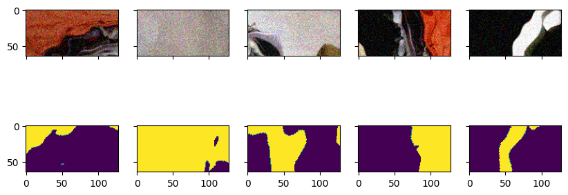
This highlights another feature of gunpowder: Requests can contain ROIs with different offsets and sizes. Internally, gunpowder will figure out what areas in the source have to be read to satisfy those heterogeneous requests, and will only read as much as needed to satisfy the request. This is useful in many applications where ground-truth is not needed for the whole input image (e.g., because of the use of valid convolutions in neural networks and the correspondingly smaller network output).

Further Example: Multiple Sources

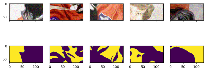
For now we assumed that both arrays we are interested in (raw and gt) are read from the same source, i.e., they are stored in the same zarr container in this example. This might not always be the case. gunpowder allows you to have multiple sources for different arrays and merge them together into one. The following example shows this functionality:

source_raw = gp.ZarrSource(
    'sample_data.zarr',
    {raw: 'raw'},
    {raw: gp.ArraySpec(interpolatable=True)}
)
source_gt = gp.ZarrSource(
    'sample_data.zarr',
    {gt: 'ground_truth'},
    {gt: gp.ArraySpec(interpolatable=False)}
)
combined_source = (source_raw, source_gt) + gp.MergeProvider()

pipeline = (
  combined_source +
  normalize +
  random_location +
  simple_augment +
  elastic_augment +
  intensity_augment +
  noise_augment +
  stack)

with gp.build(pipeline):
  batch = pipeline.request_batch(request)

imshow(batch[raw].data, batch[gt].data)

Training a network

We have seen so far how gunpowder can be used to generate training batches. In the following we will see how to train a neural network directly in this pipeline. For the example, we will train a 2D U-Net (model) on the binary ground-truth using a binary cross-entropy loss (loss). We will use PyTorch, but the same can be done with a TensorFlow model as well.

Training Preliminaries: Create Model, Loss, and Optimizer

We will use the U-Net implemention from funlib.learn.torch, but any PyTorch model can be used. To follow the example, install those packages:

pip install git+https://github.com/funkelab/funlib.learn.torch@fe60a7d9a375d64208266f96a739ab01f62a0c78
pip install torch

Here, we create a very simple 2D U-Net mapping from three channels (RGB of the raw data) to one channel (the segmentation output). The U-Net has two downsampling modules, downsampling isotropically with a factor of two. We use ‘same’ padding here, meaning that the output size of the U-Net will be the same as the input size. The number of feature maps will be four in the top-most level of the U-Net, and increase with a factor of two for each of the two following levels. The output of the U-Net is further passed through a sigmoid function to ensure values are between 0 and 1.

import torch
from funlib.learn.torch.models import UNet, ConvPass

# make sure we all see the same
torch.manual_seed(18)

unet = UNet(
  in_channels=3,
  num_fmaps=4,
  fmap_inc_factor=2,
  downsample_factors=[[2, 2], [2, 2]],
  kernel_size_down=[[[3, 3], [3, 3]]]*3,
  kernel_size_up=[[[3, 3], [3, 3]]]*2,
  padding='same')

model = torch.nn.Sequential(
  unet,
  ConvPass(4, 1, [(1, 1)], activation=None),
  torch.nn.Sigmoid())

loss = torch.nn.BCELoss()

optimizer = torch.optim.Adam(model.parameters())

Training itself is implemented in a gunpowder node, in this case torch.Train. The main benefit of using this node in a gunpowder pipeline (compared to just taking the batches we requested so far and feeding them manually to the model) is that the output of the network itself can be mapped to a gunpowder array, and subsequently be used in the pipeline. In the following, we will create a new array key prediction to do exactly that:

# create new array key for the network output
prediction = gp.ArrayKey('PREDICTION')

# create a train node using our model, loss, and optimizer
train = gp.torch.Train(
  model,
  loss,
  optimizer,
  inputs = {
    'input': raw
  },
  loss_inputs = {
    0: prediction,
    1: gt
  },
  outputs = {
    0: prediction
  })

pipeline = (
  source +
  normalize +
  random_location +
  simple_augment +
  elastic_augment +
  intensity_augment +
  noise_augment +
  stack +
  train)

# add the prediction to the request
request[prediction] = gp.Roi((0, 0), (64, 128))

with gp.build(pipeline):
  batch = pipeline.request_batch(request)

imshow(batch[raw].data, batch[gt].data, batch[prediction].data)

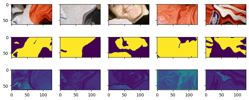
As we can see, our batch does now contain an array prediction, which is the output of the torch.Train node. This illustrates another feature of gunpowder: Arrays can be generated by any node, this functionality is not limited to source nodes (and in fact, source nodes are in no way special, they are simply gunpowder nodes that do not require an input and provide an array).

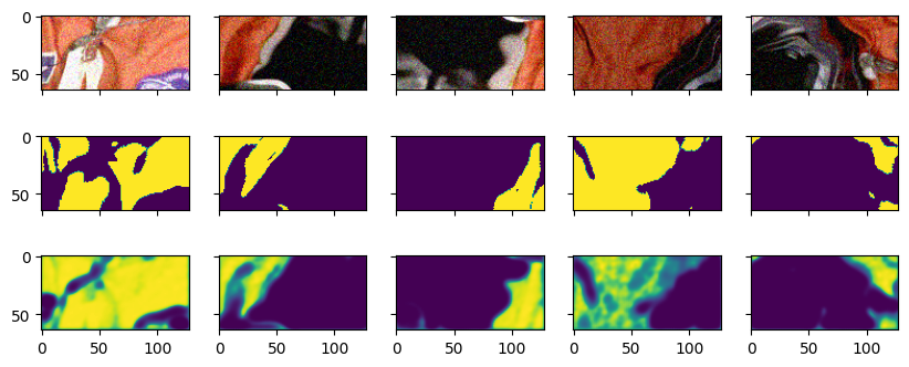
But the train node above did not just produce a prediction: Since we also told it which loss and optimizer to use, and since we linked the output of our network and the ground-truth to the loss via loss_inputs, the train node did also perform a training iteration for us. This becomes more evident if we keep training for a few iterations:

with gp.build(pipeline):
  for i in range(1000):
    batch = pipeline.request_batch(request)

imshow(batch[raw].data, batch[gt].data, batch[prediction].data)

Note

The predictions are only included in the batch because we requested them here to visualize them. To keep the example simple, we request the predictions in every iteration. In a production setting, however, it is advisable to request only what is needed for each iteration. This saves a potentially expensive copy from GPU memory.

Predicting on a whole image

gunpowder and its pipeline concept can not just be used for training, but also to perform the final predictions once training is finished. The following example shows how to assemble a pipeline to take the model we just trained and apply it on the whole image. The main difficulty in doing that is that the model was trained for a particular input size. Consequently, the whole image will have to be chunked into pieces of the correct size, and the network has to be applied to each chunk in a scanning fashion, creating predictions one chunk at a time. Those chunks then have to be reassembled into a prediction for the whole image. This whole procedure is orchestrated by another gunpowder node: Scan.

# set model into evaluation mode
model.eval()

predict = gp.torch.Predict(
  model,
  inputs = {
    'input': raw
  },
  outputs = {
    0: prediction
  })

stack = gp.Stack(1)

# request matching the model input and output sizes
scan_request = gp.BatchRequest()
scan_request[raw] = gp.Roi((0, 0), (64, 128))
scan_request[prediction] = gp.Roi((0, 0), (64, 128))

scan = gp.Scan(scan_request)

pipeline = (
  source +
  normalize +
  stack +
  predict +
  scan)

# request for raw and prediction for the whole image
request = gp.BatchRequest()
request[raw] = gp.Roi((0, 0), (512, 512))
request[prediction] = gp.Roi((0, 0), (512, 512))

with gp.build(pipeline):
  batch = pipeline.request_batch(request)

imshow(batch[raw].data, None, batch[prediction].data)

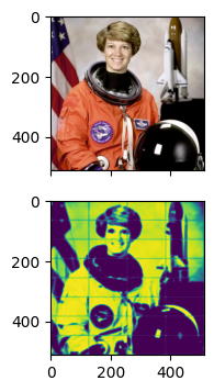
The main difference to the training pipeline used earlier is that there is no longer a need for data augmentation. We also replaced the torch.Train node with its equivalent torch.Predict.

Further Example: Prediction in Large nD Arrays

Here, we make a request to Scan for the whole image and the prediction. This is fine as long as both arrays are small enough to fit into memory. However, gunpowder was designed to work with arbitrarily large nD arrays. Therefore, Scan accepts empty requests as well, which will still result in small scan_request s being performed in a scanning fashion over the whole input range–the only difference is that Scan does not keep the individual results and consequently that the batch returned by Scan will be empty.

So how do we get access to the prediction then to store it, for example, in a zarr container? The answer is to add a node between predict and scan, through which every batch will pass before it is being discarded. The ZarrWrite node will, for instance, assemble a zarr container of all the arrays passing through it.

The following example illustrates that:

# prepare the zarr dataset to write to
f = zarr.open('sample_data.zarr')
ds = f.create_dataset('prediction', shape=(1, 1, 512, 512))
ds.attrs['resolution'] = (1, 1)
ds.attrs['offset'] = (0, 0)

# create a zarr write node to store the predictions
zarr_write = gp.ZarrWrite(
  output_filename='sample_data.zarr',
  dataset_names={
    prediction: 'prediction'
  })

pipeline = (
  source +
  normalize +
  stack +
  predict +
  zarr_write +
  scan)

# request an empty batch from scan
request = gp.BatchRequest()

with gp.build(pipeline):
  batch = pipeline.request_batch(request)

print(batch)
imshow(
  zarr.open('sample_data.zarr')['raw'][:],
  None,
  zarr.open('sample_data.zarr')['prediction'][:])

What next?

gunpowder provides much more nodes to chain together, including a pre-cache node for easy parallel fetching of batches, several augmentation nodes, and nodes for profiling and inspection. For a complete list see the API reference.