What's in a QuAC?
Prologue
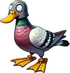
Note: Everything here is human, fly, and microscope-generated, except for the portrait of Simon which is DALL-E-generated.
Simon’s Quest
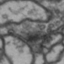
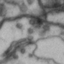
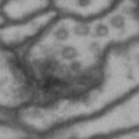
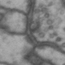
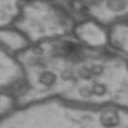
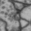
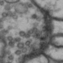
While it is obvious that Simon is a duck, there are certain instances of such categorization that are not so obvious. Take for instance these images of synapses in the fruit fly brain.
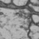
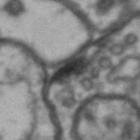
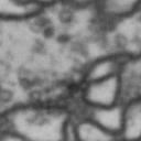
Read more: Synapse and neurotransmitters
The brain of a fruit fly, just like that of a human, contains many cells called neurons. These neurons are connected together in places called synapses. At the synapses, the neurons are able to communicate with each other, though usually only in one direction. The pre-synaptic neuron emits the messages, and the post-synaptic neurons receives them. The communication at these synapses happens via an exchange of neurotransmitters, small molecules that are able to go from one cell to another at the synapse. Each neurotransmitter will have a slightly different message; for example some neurotransmitters will activate the post-synaptic neurons, while others inhibit them. In the fly, some will do both.By combining many complex, painstakingly implemented biological experiments, we are able to say that some of these synapses release acetylcholine (or ACh, for short), while others release dopamine. Unfortunately, we can’t really tell from looking at them. This is frustrating, because there are hundreds of millions of synapses in the fruit-fly’s brain, and running an experiment for each one to figure out what it’s emitting would be both difficult and expensive.
Read more: See the images with labels
Acetylcholine
Dopamine


In this story, we look at two specific neurotransmitters: acetylcholine and dopamine. However, we can, and have, applied this process to a group of six different neurotransmitters: GABA, acetylcholine, glutamate, serotonin, octopamine, and dopamine.
Luckily, Simon’s colleagues in the Funke Lab found that if you use the synapses whose neurotransmitter types you do know as training data, you can get an artificial neural network to predict the type of neurotransmitter of synapses it has never seen before (Eckstein et al., 2024) And most of the time… it was right!
But Simon and his colleagues were wary. How could it possibly know? Simon had looked at thousands of synapses before, and he couldn’t even tell the difference. What could the classifier be looking at, and was it even real? And look here, people said, it may be right most of the time, but it keeps saying Kenyon cells use dopamine when we all know they use ACh! Surely, the only explanation for this is that the classifier doesn’t know what it is doing… right? So with his classifier in hand, Simon decided he had to venture into a dangerous, uncharted realm: the land of explainable AI.
Into the land of XAI
As he ventured in, Simon saw a stone path laid in front of him and decided to follow it. He walked until he saw a sign:
Inherently Interpretable Only
No pre-trained classifiers allowed!
He stopped at the threshold for a while, looking into the village in the glade before him. Before each house was a sign, similar to the one in front of him. On each, a different constraint was placed: “Trees only”, “Assumed gaussian”, “Concepts required”. Looking into his bag at his very own tools, his data and his classifier, he sighed. It fit none of those requirements, and he would not be welcome here. Undeterred he decided to place the village on his map, turn around, and move on.
Read more: Inherently interpretable models
The field of XAI is young and rapidly evolving. It has many factions, including that of inherently interpretable models. These models are built with specific assumptions in mind, and specific requirements on both the task and the data to make a model whose inner functioning can be directly understood rather than extracted later as we do here. Examples span from random forest models to the ProtoPNet (Chen et al., 2019).In our work we focused instead on post-hoc explainability: where you already have a trained model that works and you try to make sense of it after it is done. There are many reasons to do post-hoc explainability. Sometimes, the requirements for an inherently interpretable model are not satisfied in your case. Often, an inherently interpretable model will also be less powerful than a standard black-box model, because of the additional constraints. Or you just have a functional model already that you want to use irrespective of its interpretability, and are curious as to how it works.
Stepping off of the stone path, he decided to take a side trail that he had seen on the way out. It was not so orderly as the previous path had been, but it looked to have been travelled by many before him. Eventually, he arrived at a clearing in the trees. Several people were sat around a fire, in a somewhat chaotic-looking campsite. Unlike the village he had just left, these people seemed very welcoming.
Simon walked in and introduced himself, and described his problem. He brought out his data and his classifier, and explained that he wanted to understand how his classifier knew what type each synapse was by looking at the image. At once, each person in the glade started taking out inspection tools. They were all similar tools in principle, but with very different embellishments and scopes and levers. The people in the glade called these tools attribution methods.
Read more: Attribution methods
An attribution method in the realm of image classification is a method that, given an image (and usually a target class) will output a heatmap to describe how important any given pixel of the input image is for the classifier's output. Many attribution methods do this by looking at the gradients of the model at the input image. This is problematic for many standard classification models, whose gradients are quite noisy (even to changes that are imperceptible to the human eye). It is also problematic for cases of "perfect classifications", where the classifier is so convinced of a given classification that there are no gradients remaining. In those cases, some attribution methods will try to do a comparison between the image and a baseline, such as a blank image or an image of gaussian noise. In those cases, the choice of the baseline is particularly important.Finally, in our hands, existing attribution methods have returned very different interpretations. Most of these have not been biologically interpretable or testable. The main reason for this is that even when they return a reasonable region as an output, they have no way of telling us why that region was important. Without the counterfactual as a comparison, we are therefore missing valuable information.
They passed the data and classifier among them. They took the classifier’s gradients, they compared the images to empty images, they compared them to noise, they pulled out internal activations… each of them diligently going through until they were satisfied. “Yes,” they said, “we can use our tools to tell you how the classifier knows what type each image is.”
Excited, Simon chose one example and asked: “so what makes this synapse ACh?”. The response was underwhelming. Each of the attribution methods had returned a slightly different answer. Some of them had even highlighted the entire synapse. He wasn’t really sure what to make of this. Still, he rallied himself, chose one person at random, and asked: “You say this region is what makes this synapse ACh… why?”. “Easy,” they answered, “that is where the classifier’s gradients are strongest!”
“But…”, said Simon, “why this part? Does this part look different in dopamine?”. His only response was a shrug. Still… it was a welcoming glade, so he stayed awhile. Each of his new friends taught him how to make their tool until he was left with a collection of attribution methods to choose from. When he had collected as many of them as he could carry, he finally decided to keep going.
Next, he ventured even further, until he left the forest and reached a wide plain. In the distance he saw a set of brightly colored caravans. He approached, and saw that a strange motto was painted on the side of many of the wagons:
Change reality!
Curious, he went forth and introduced himself once again. It was a traveling performance troupe, a small family of actors, each more exuberant than the last. He introduced himself and his quest once again, and brought out his data and his tools. Ignoring the tools, the Matriarch of the family took a keen interest in the data. She had her children and grandchildren sort it into piles: one for ACh and one for dopamine.
“If you want to know the difference between the synapses in the two piles”, she said, “you need to learn how to move an item from one to the other”. Simon was perplexed, how could you move an ACh synapse to dopamine? It was what it was, wasn’t it?
The Matriarch grinned and said “Watch this”. Then she pulled one image from the top of the ACh pile and transformed it! Parts of the image had changed from what they were before. She gently asked Simon if she could borrow his classifier, and put this new image into it. In went what had been an ACh image, and the verdict? It was now dopamine!
Simon was delighted, and ran to pick up both images: the real one, and the new one that the matriarch had just generated. They were different, but also the same… They looked as though they were the same synapse in two different outfits.
Read more: Generating counterfactual candidates
The task of transforming images from one type, or domain, to another is often called domain transfer. In recent years, one effective way of doing domain transfer has been generative models, specifically conditional generative models. These models take an input, and are trained to transform it into the same input of a different type or domain.The specific generative model that we used for this project is a StarGAN (Choi et al., 2020). The StarGAN is an example of a Generative Adversarial Model, so named because their training process involves pitting two neural networks against each other. A generator will be trained to make modifications to the image, and a discriminator is simultaneously trained to distinguish real images from generated images. The goal of the generator is to create images that are realistic enough to fool the discriminator.
In the case of domain transfer, the discriminator needs to specifically recognize real images of a given type from fake images of that type. This means that it is not enough for the generator to create realistic images, it needs to create realistic images that have the features of a given domain or type.
As a concrete example, say we give the generator an ACh image, and dopamine as a target. It will modify that image slightly --- not too much that it can't recover the original image if brought back the other way. Then the discriminator will judge the image. Does it look real? Does it look like dopamine? If both of those conditions are met, it will confirm that this is a real image, marking a success for the generator!
Generative models aren't perfect, however. Although we regularize our StarGAN to avoid making unnecessary changes, sometimes it still produces unnecessary artifacts as a side-product of the conversion, which we need to learn how to deal with later.
“So these are the differences between ACh and dopamine?” he asked the Matriarch. “These changes turn ACh into dopamine, certainly. I might have added some embellishments,” she responded. Simon’s spirits sank the tiniest bit. “Where?”, he asked. The Matriarch laughed at that question: “Who’s to say?”
Simon decided to stay and learn the craft of conversion from the people in the caravan. It was a much harder task than he had initially expected. He had to keep a delicate balance, or what he generated ended up either too similar to the real image that he had started with, or so different as to be unrecognizable. At one point, all he went so over the top that everything that he generated ended up looking the same, no matter what he put in! Eventually, he did figure it out. And so it was that, with hearty goodbyes from the Matriarch and her colorful family, he continued on his journey.
Building QuAC
Having reached what seemed to be the end of the explored path, Simon arrived at a small beach near a lake so wide that he could barely see the other side. There, he set himself up with a small shelter, laid out in front of him all that he had learned, and got to work. First, he got to work converting all of his ACh images into dopamine and vice versa. He was meticulous, and tested his conversions with his classifier. Sometimes, he had to try generating multiple options for a given image before he found one that would satisfy the classifier. Still, by the end he was reasonably happy that he had been able to convert a majority of his synapses from one type to the other.
Then, he needed to find a way to remove the “embellishments” that the Matriarch had talked about. She had not had a way of telling him what they were, but he had other tools at his disposal! Looking at his attribution methods, Simon realized that if he modified those just so, they would be able to tell him which of the differences between his images were important to tell the difference between ACh and dopamine, and which ones he could ignore.
Read more: Discriminative attribution methods
Discriminative attribution methods are a slight extension of existing attribution methods where instead of asking the question "which region of this image is important for this class" we ask "which region of difference between these two images is important for the difference between these two classes?"Let's take the example of integrated gradients (Sundararajan et al., 2017). This attribution method is normally defined as the integral of the gradients of the network, over a path from a blank baseline \(x_0\) to the query image \(x\). \( IG(x) = (x - x_0) \int_{\alpha=0}^{1}\frac{\partial f(x_0 + \alpha(x - x_0))}{\partial x}\partial\alpha \) To modify this, and make it discriminative, we simply use the generated image \(x_g\) as a baseline instead. \( DIG(x) = (x - x_g) \int_{\alpha=0}^{1}\frac{\partial f(x_g + \alpha(x - x_g))}{\partial x}\partial\alpha \) We evaluate both of these at the real class.
With his new discriminative attribution methods, Simon was on a roll. “Now all I need”, he thought to himself, “is to decide which tool to choose for the job.” He pondered for a while. “It needs to be the tool that gives me the minimal change with the maximum effect,” he continued. He created an attribution mask from the discriminative attribution by choosing a level of importance and setting it. Then he cut out that specific part from the generated image, and added it into the real ACh image. Looking at the result, he saw that it still looked quite like a synapse, so he fed it to the classfier. The classifier noticed the change, certainly, but not enough to say it was now dopamine. So he tried a different importance level, and iterated.
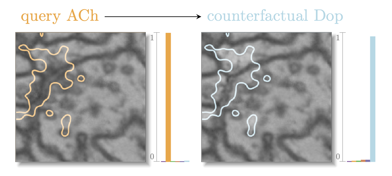
Eventually, he had tried 100 different importance levels for each of his tools until he finally found what he was looking for. With the construction, he had made a minimal change to his real image with a maximal effect on the classifier. He had made a counterfactual. This is what it looked like:
Read more: The QuAC method
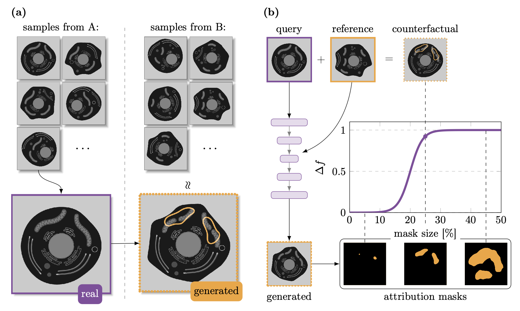 QuAC, or Quantitative Attributions with Counterfactuals (Adjavon et al., 2024), is a method for generating and scoring visual counterfactual explanations of an image classifier. We currently assume in QuAC that there are images of different conditions, though it can be more than two conditions, and that a classification task is solvable with reasonable performance by a pre-trained classifier. We use an artificial neural network as a classifier, but it can be any function that takes an image as input and returns a normalized score for each of the classes.
 We begin by training a generative neural network (we use a StarGAN (Choi et al., 2020)) to convert the images from one class to another. This allows us to go from our real query image, to a generated image. Using information learned from reference images, the StarGAN is trained in such a way that the generated image will have a different class.
While very powerful, generative networks can potentially make some changes that are not necessary to the classification. In the example in the figure, the generated image’s membrane has been unnecessarily changed. We use discriminative attribution methods to generate a set of candidate attribution masks. Among these, we are looking for the smallest mask that has the greatest change in the classification output. By taking only the changes within that mask, we create the counterfactual image. It is as close as possible to the original image, with only the necessary changes to switch its class.
The visual explanations that we provide can be scored by their effect on the classifier's output. We find that, by looking at the top-scored samples, we can name putative features that make one class different from the others. In benchmarks with known features, we have been able to recover them using this method. In other cases, we have found features that could be verified experimentally, many of which have plausible biological explanations.
While we've currently only applied QuAC to images, the same principles and set of steps could be applied to a variety of different data types, and we hope to explore this soon!
Now, he could begin to see something! Working through the night, he did the same thing for all of the synapses in his pile: in one direction, then the other. When an example had a particularly strong effect on the classifier, with a particularly small attribution mask he put it to the top of his final pile to look at it first later. Some examples he relegated to the bottom of his pile.
Epilogue
When dawn came, Simon had looked at about a hundred images in detail, and from the first ten he was already getting a good grasp of what would convince his classifier. The cleft of the synapse was getting shorter, the post-synaptic densities were changing, some vesicles were changing size… he could even already think of a biological reason for some of these things. Something he could test!
This was when he finally decided to pull out his ultimate test… the one he had been afraid to look at this whole time: he extracted his Kenyon cell synapses. Now, he knew that the classifier was wrong about these: they were ACh, but the classifier really thought they were dopamine. Still, he thought maybe if tried the process in the opposite direction — turning them back into the correct type — he would figure out why that was. And there it was again: the cleft, the vesicles, the post-synaptic densities… Suddenly he had a new hypothesis: what if the Kenyon cells really do look like dopamine? Excited to put his ideas to the test, he packed up all of his newfound tools, and carefully balanced his pile of images in order. Then, picking up his map, he began his return journey.
Read more: The Kenyon cells
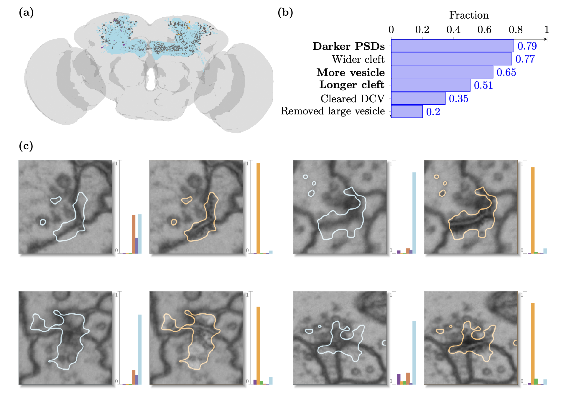 Kenyon cells are a group of neurons in the fly Mushroom Body, which are involved in the olfactory system: how the fly smells. They are well studied, and are known to release acetylcholine as a small-molecule neurotransmitter. In all of our experiments, however, the synapses of Kenyon cells were overwhelmingly classified as dopaminergic.
 To try to explain this, we decided to try to apply QuAC in reverse. If the classifier was saying than an image was dopaminergic, how could we switch it back to the correct clasification of ACh? We looked at 100 highly scored explanations and annotated the changes that we saw going from dopaminergic to cholinergic for Kenyon cells. Several of these features were quite prevalent, among which three (bolded in the histogram in the figure above) that had already been found to be a difference between acetylcholine and dopamine in cases where the classifier was correct. In other words, it seems like the Kenyon cells really do look dopaminergic --- at least they look more like the dopaminergic synapses in our training dataset than the cholinergic ones.
Several of the features we found relate to known phenomena that can be empirically tested. One such example is the length (not width) of the synaptic cleft. In flies, where synapses can be one-to-many, a longer cleft relates to more post-synaptic partners. Since we have the connectome of the fly, which describes all connections in the brain, we can count the number of post-synaptic partners for our training dataset (separately, per-class), then count the number for Kenyon cells. If we're right, biologists can start digging into why Kenyon cells would need to differ in this way from other cholinergic neurons.
So it was that Simon returned home. As he turned to look back on the wide world of XAI, he beamed. Where he had previously only seen danger and the unknown, now he could see all of the future adventures that lay before him. He still didn’t know exactly what made the difference between synapses that look like ACh and synapses that look like dopamine, but he had some ideas. More importantly, now he had all the tools that he needed to find out.
References
- arXiv:1806.10574 [cs, stat], Dec 2019

